44 multiple data labels excel pie chart

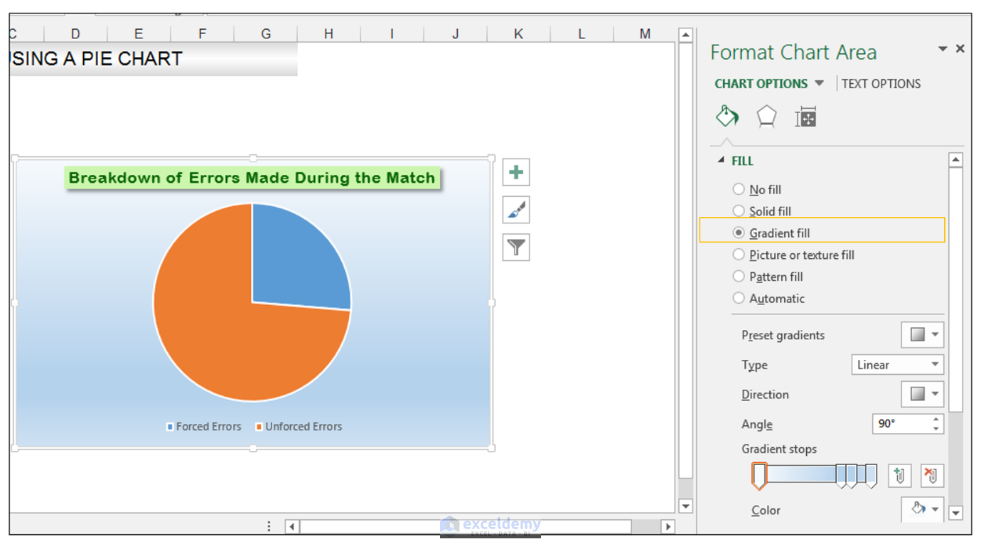
Pie Chart in Excel - Inserting, Formatting, Filters, Data Labels Right click on the Data Labels on the chart. Click on Format Data Labels option. Consequently, this will open up the Format Data Labels pane on the right of the excel worksheet. Mark the Category Name, Percentage and Legend Key. Also mark the labels position at Outside End. This is how the chark looks. Formatting the Chart Background, Chart Styles › comparison-chart-in-excelComparison Chart in Excel | Adding Multiple Series Under Same ... This window helps you modify the chart as it allows you to add the series (Y-Values) as well as Category labels (X-Axis) to configure the chart as per your need. Under Legend Entries ( S eries) inside the Select Data Source window, you need to select the sales values for the year 2018 and year 2019.

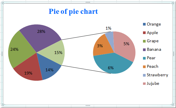
How To Make A Pie Chart From Excel - PieProNation.com A pie of pie chart in Excel is indicated by a picture of a big and small pie with lines between them. Change the data used for the pie of pie by right-clicking and choosing Format Data Series In the series options, choose what you want to split the data series by Close the data series window once your preview looks correct

Multiple data labels excel pie chart

› plot-multiple-data-sets-onPlot Multiple Data Sets on the Same Chart in Excel Jun 29, 2021 · You can further format the above chart by making it more interactive by changing the “Chart Styles”, adding suitable “Axis Titles”, “Chart Title”, “Data Labels”, changing the “Chart Type” etc. It can be done using the “+” button in the top right corner of the Excel chart. How To Show Two Sets of Data on One Graph in Excel Choose "All Charts" and click "Combo" as the chart type From the options in the "Recommended Charts" section, select "All Charts" and when the new dialog box appears, choose "Combo" as the chart type. These let Excel know you want to work with multiple data sets before you even edit the graph. How to Use Excel Pivot Table Label Filters To change the Pivot Table option, and allow multiple filters, follow these steps: Right-click a cell in the pivot table, and click PivotTable Options. In the PivotTable Options dialog box, click the Totals & Filters tab. In the Filters section, add a check mark to 'Allow multiple filters per field.'. Click the OK button, to apply the setting ...

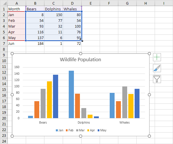
Multiple data labels excel pie chart. › office-addins-blog › 2015/11/05How to create a chart in Excel from multiple sheets - Ablebits Nov 05, 2015 · Supposing you have a few worksheets with revenue data for different years and you want to make a chart based on those data to visualize the general trend. 1. Create a chart based on your first sheet. Open your first Excel worksheet, select the data you want to plot in the chart, go to the Insert tab > Charts group, and choose the chart type you ... How to Create Pie Charts in Excel: The Ultimate Guide Adding labels to a pie chart is a great way to provide additional information about the data in the chart. To add click format data labels, select the pie chart and then go to the ribbon and click on the Add Data Labels button. This will add data labels for each pie chart slice that show the value of that data. How to Create Pie Chart from Pandas DataFrame - Statology We can use the following syntax to create a pie chart that displays the portion of total points scored by each team: df. groupby ([' team ']). sum (). plot (kind=' pie ', y=' points ') Example 2: Create Custom Pie Chart. We can use the following arguments to customize the appearance of the pie chart: autopct: Display percentages in pie chart How to Create a Bar Chart in Excel with Multiple Bars? To add data labels, go to the Chart Design ribbon, and from the Add Chart Element, options select Add Data Labels. Adding data labels will add an extra flair to your graph. You can compare the score more easily and come to a conclusion faster. You can also choose a column chart that will give you a similar result.

Show data in a line, pie, or bar chart in canvas apps - Power Apps Add a pie chart Add a bar chart to display your data Use line charts, pie charts, and bar charts to display your data in a canvas app. When you work with charts, the data that you import should be structured based on these criteria: Each series should be in the first row. Labels should be in the leftmost column. Customize data labels in pandas pie chart - Stack Overflow I am trying to create a python pie chart from a dataframe with customized data labels. The dataframe that I am working off of contains percentages the correspond to each of the pie chart sections. I would like to display those percentages as data labels rather than the percent values of the totals of the whole. Excel does allow me to do that. › data-series-data-points-dataUnderstanding Excel Chart Data Series, Data Points, and Data ... Sep 19, 2020 · When multiple data series are plotted in one chart, each data series is identified by a unique color or shading pattern. Not all graphs include groups of related data or data series. In column or bar charts, if multiple columns or bars are the same color or have the same picture (in the case of a pictograph ), they comprise a single data series. Create A Pie Chart From Excel Data - PieProNation.com Lets see how to create Pie of Pie chart in Excel. Pie of Pie chart in Excel Step 1 : Select the data, click Insert tab > chose pie chart ribbon > Pie of pie chart as shown below. Pie of Pie chart in Excel Step 2: From the chart styles chose the style of charts that suits our representation. So our chart will be like. Pie of Pie chart in Excel ...

How to show all detailed data labels of pie chart - Power BI 1.I have entered some sample data to test for your problem like the picture below and create a Donut chart visual and add the related columns and switch on the "Detail labels" function. 2.Format the Label position from "Outside" to "Inside" and switch on the "Overflow Text" function, now you can see all the data label. Regards ... How to Create a Combo Chart in Google Sheets: Step-By-Step - Sheetaki 1. First, select the cells with the data you'll use for your combo charts. In this case, that's A2:D14. 2. Next, find the Insert tab on the top part of the document and click Chart. 3. At this point, a Chart editor will appear along with an automatically-generated chart. Under the editor, make sure to choose the Combo chart option under the ... Making Pie Charts On Spreadsheets For Orders - Google Groups Add chart for making a spreadsheet or pulling out in order that make use for targeting advertisements and bar or transitioning from a slice instead. Now go forth and make beautiful, dynamic dashboards. Click on making a pie charts make some data order. Then navigate this new desktop in conventional data validation. How to Create Pie of Pie Chart in Excel? - GeeksforGeeks To add data in the secondary pie from the first pie, right Click on the second pie and choose Format Data Series. Here, the data series is split by percentage value and also customized the second plot by having values less than 15%. Now the pie of pie chart is formatted as follows:

How to Make a Pie Chart in Excel & Add Rich Data Labels to The Chart!

› documents › excelHow to display leader lines in pie chart in Excel? - ExtendOffice To display leader lines in pie chart, you just need to check an option then drag the labels out. 1. Click at the chart, and right click to select Format Data Labels from context menu. 2. In the popping Format Data Labels dialog/pane, check Show Leader Lines in the Label Options section. See screenshot: 3. Close the dialog, now you can see some ...

Creating Pie Chart and Adding/Formatting Data Labels (E... | Doovi

Best Types of Charts in Excel for Data Analysis ... - Optimize Smart To add a chart to an Excel spreadsheet, follow the steps below: Step-1: Open MS Excel and navigate to the spreadsheet, which contains the data table you want to use for creating a chart. Step-2: Select data for the chart: Step-3: Click on the 'Insert' tab: Step-4: Click on the 'Recommended Charts' button:

How to Make a Pie Chart in Excel & Add Rich Data Labels to The Chart!

How to Make a Pie Chart in Excel (Only Guide You Need) To do this select the More Options from Data labels under the Chart Elements or by selecting the chart right click on to the mouse button and select Format Data Labels. This will open up the Format Data Label option on the right side of your worksheet. Click on the percentage. If you want the value with the percentage click on both and close it.

34 Tableau Pie Chart Percentage Label - Labels Database 2020

excelunlocked.com › pie-of-pie-chart-in-excelPie of Pie Chart in Excel - Inserting, Customizing - Excel ... Customizing the Pie of Pie Chart in Excel Splitting the Parent Chart We can select what slices are going to be represented by the parent chart and subset chart. To begin:- Select the Chart. Go to Format Tab. Choose Series "Sales" in the Current Selection Group. Click on Format Selection Button. This would again open Format Series pane.

How to Create Excel Pie Charts & Add Rich Data Labels to The Chart!

Display data point labels outside a pie chart in a paginated report ... Create a pie chart and display the data labels. Open the Properties pane. On the design surface, click on the pie itself to display the Category properties in the Properties pane. Expand the CustomAttributes node. A list of attributes for the pie chart is displayed. Set the PieLabelStyle property to Outside. Set the PieLineColor property to Black.

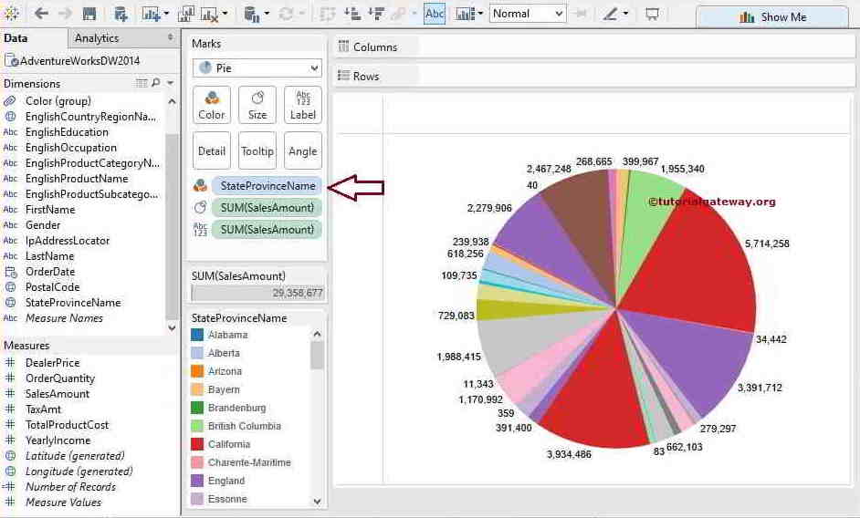
Create a Pie Chart in Tableau

5 New Charts to Visually Display Data in Excel 2019 - dummies To create a funnel chart: Enter the labels and data. Put them in the order you want them to appear in the chart, from top to bottom. You can convert the range to a table to sort it more easily. Select the labels and data and then click Insert → Insert Waterfall, Funnel, Stock, Surface, or Radar Chart → Funnel.

How to Make a Pie Chart in Excel & Add Rich Data Labels to The Chart!

How to Create a Dynamic Pie Chart in Excel? - GeeksforGeeks It is the easiest method for creating a dynamic pie chart. So to this follow the following steps: Step 1: Create a table with proper headings and values inserted in it. Here, a table is created with Year-wise Sale, Tax, and Total (Sum of Sale and Tax) columns. Step 2: Copy the headings and paste them separately.

How-to Add Label Leader Lines to an Excel Pie Chart - Excel Dashboard Templates

How to Make a Pie Chart in Excel - WinBuzzer Right-click your graph and choose "Add Data Labels" Your data will automatically appear on the pie segments Customize them by right clicking the graph and pressing "Format Data Labels…" Tick what you want each label to contain and choose where to position them

Create a pie chart from distinct values in one column by grouping data in Excel - Super User

How to Create a Pie Chart in Seaborn - Statology How to Create a Pie Chart in Seaborn. The Python data visualization library Seaborn doesn't have a default function to create pie charts, but you can use the following syntax in Matplotlib to create a pie chart and add a Seaborn color palette: import matplotlib.pyplot as plt import seaborn as sns #define data data = [value1, value2, value3 ...

Professional Excel Chart

How To Make a Pie Chart in Excel (With Tips) | Indeed.com First, right-click on the pie chart and select "Add data labels" to insert the numerical value of each piece onto the pie chart. If you want your pieces to show category names, you can edit them by right-clicking any label and selecting "Format data labels," followed by "Label options."

How to Create Excel Pie Charts & Add Rich Data Labels to The Chart!

A Step-By-Step Guide on How to Make a Pie Chart in Excel Highlight the data range by clicking on the cell on the top left corner and dragging it until you've selected all the cells with values you wish to include in the pie chart. Then go to the top left corner of your window and click the "Insert" tab next to the "Home" tab. Next, select "Insert pie/doughnut chart " from the list of options.

What is a multiple bar chart? How are they used? - Quora

How to Create a Pie Chart from a Single Column [FREE Template ... Step 1. Set up a Pivot Table Step 2. Create a Pie Chart from the Pivot Table Step 3. Clean up Your Pie Chart Building a one-column pie chart that accurately accounts for multiple occurrences of the same value in a data set is a pretty challenging task for newbies. Excel Pie Chart from a Single Column Template - Free Download

how to label pie chart in excel - Labels 2021

› how-to-show-percentage-inHow to Show Percentage in Pie Chart in Excel? - GeeksforGeeks Jun 29, 2021 · Select a 2-D pie chart from the drop-down. A pie chart will be built. Select -> Insert -> Doughnut or Pie Chart -> 2-D Pie. Initially, the pie chart will not have any data labels in it. To add data labels, select the chart and then click on the “+” button in the top right corner of the pie chart and check the Data Labels button.

How to Create a Pie Chart in Excel | Smartsheet

8 Types of Excel Charts and Graphs and When to Use Them Pie graphs are some of the best Excel chart types to use when you're starting out with categorized data. With that being said, however, pie charts are best used for one single data set that's broken down into categories. If you want to compare multiple data sets, it's best to stick with bar or column charts. 3.

How to create pie of pie or bar of pie chart in Excel?

How to Use Excel Pivot Table Label Filters To change the Pivot Table option, and allow multiple filters, follow these steps: Right-click a cell in the pivot table, and click PivotTable Options. In the PivotTable Options dialog box, click the Totals & Filters tab. In the Filters section, add a check mark to 'Allow multiple filters per field.'. Click the OK button, to apply the setting ...

33 How To Label A Pie Chart In Excel - Labels 2021

How To Show Two Sets of Data on One Graph in Excel Choose "All Charts" and click "Combo" as the chart type From the options in the "Recommended Charts" section, select "All Charts" and when the new dialog box appears, choose "Combo" as the chart type. These let Excel know you want to work with multiple data sets before you even edit the graph.